Basics#

Notebook showing a fast and efficient way to load Sentinel-2 L1C data into xarray

import glob
import os
import numpy as np

import pandas as pd
import geopandas as gpd
import xarray as xr

import matplotlib.pyplot as plt
import matplotlib as mpl
import cartopy.crs as ccrs
from matplotlib.colors import ListedColormap

import memory_profiler

import GRSdriver
from GRSdriver import driver_S2_SAFE as S2

%load_ext memory_profiler

opj = os.path.join

GRSdriver.__version__

'1.0.5'

Set the path of the images you want to load, here is a example for the former (v3) and current (v4) image formatting#

imageSAFE ='/data/satellite/S2/cnes/S2B_MSIL1C_20220811T100559_N0400_R022_T31NDH_20220811T171744.SAFE'
imageSAFE ='/home/harmel/Dropbox/Dropbox/satellite/S2/L1C/S2B_MSIL1C_20230711T030529_N0509_R075_T49QDB_20230711T054244.SAFE'

First, check the availbale bands:#

GRSdriver.driver_S2_SAFE.INFO

bandId	0	1	2	3	4	5	6	7	8	9	10	11	12
ESA	B01	B02	B03	B04	B05	B06	B07	B08	B8A	B09	B10	B11	B12
EOREADER	CA	BLUE	GREEN	RED	VRE_1	VRE_2	VRE_3	NIR	NARROW_NIR	WV	SWIR_CIRRUS	SWIR_1	SWIR_2
Wavelength (nm)	443	490	560	665	705	740	783	842	865	945	1375	1610	2190
Band width (nm)	20	65	35	30	15	15	20	115	20	20	30	90	180
Resolution (m)	60	10	10	10	20	20	20	10	20	60	60	20	20

Choose the bands to be loaded (fill the bandIds array up) and the resolution between 10, 20 and 60 m:#

bandIds = [0,1,2,3,8,11]
resolution=60

Create the s2driver objects for the selected images#

l1c = S2.Sentinel2Driver(imageSAFE,band_idx=bandIds,resolution=resolution)

If you want to get the radiometric bands only (i.e., top-of-atmosphere reflectance)#

%time %memit l1c.load_bands()

peak memory: 3138.26 MiB, increment: 1731.34 MiB
CPU times: user 4min 34s, sys: 7.48 s, total: 4min 42s
Wall time: 18.2 s

/home/harmel/anaconda3/envs/grstbx/lib/python3.9/site-packages/xarray/core/indexes.py:659: RuntimeWarning: '<' not supported between instances of 'SpectralBandNames' and 'SpectralBandNames', sort order is undefined for incomparable objects.
  new_pd_index = pd_indexes[0].append(pd_indexes[1:])

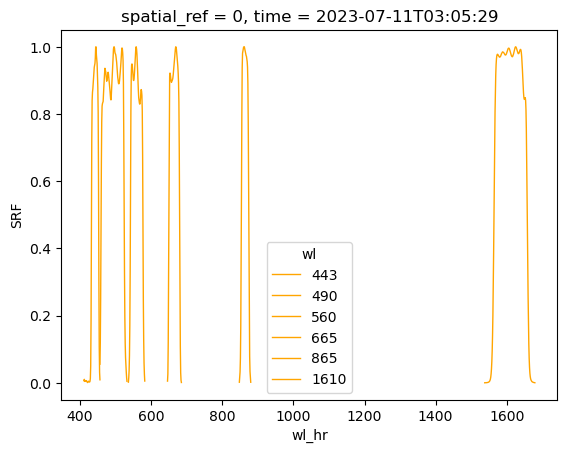
From that stage you can check some metadata such as crs or spectral response functions:#

print(l1c.prod.rio.crs)
l1c.prod.SRF.plot(x='wl_hr',hue='wl',color='orange',lw=1)

EPSG:32649

[<matplotlib.lines.Line2D at 0x7f3fd0a06160>,
 <matplotlib.lines.Line2D at 0x7f3fd0a063a0>,
 <matplotlib.lines.Line2D at 0x7f3fd0a06490>,
 <matplotlib.lines.Line2D at 0x7f3fd0a06520>,
 <matplotlib.lines.Line2D at 0x7f3fd0a065e0>,
 <matplotlib.lines.Line2D at 0x7f3fd0a066d0>]

../_images/81ab36420e38bb163082f9999eb65a6f429ebd468118e9207d8d3066905b37e3.png

Plotting section#

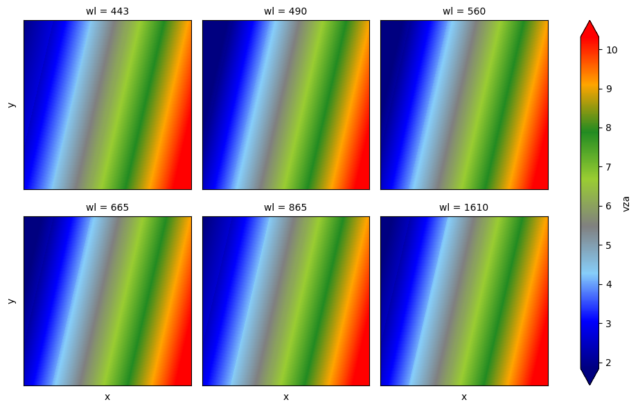
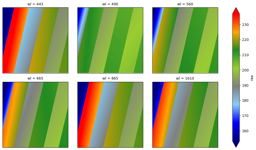
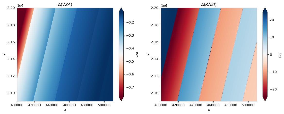
The MSI-Sentinel-2 instrument is composed of 12 detectors staggered in two different rows making a “switch” in viewng geometries along the image especially for the azimuth values. Here, we plot the solar and viewing zenith angles as well as the relative azimuth between Sun and sensor directions. The sun viewing angle (SZA) is common to all the spectral bands.

The sensor angles are dependent on the spectral band considered, here are the viewing zenith angle (VZA) and the relative azimuth (RAZI) for the bands loaded in the S2 object.

VZA#

cmap = mpl.colors.LinearSegmentedColormap.from_list("",['navy', "blue", 'lightskyblue', 'gray', 'yellowgreen', 'forestgreen', 'orange', 'red'])
fig = l1c.prod.vza.plot.imshow(col='wl', cmap=cmap, col_wrap=3,  robust=True,subplot_kws=dict(xlabel='',xticks=[], yticks=[]))

../_images/59179bf70e95d7a34c85a4f927713e655faa8d45894f2f06e9cd9614ef943dd2.png

RAZI#

import cartopy.crs as ccrs
str_epsg = str(l1c.prod.bands.rio.crs)
zone = str_epsg[-2:]
is_south = str_epsg[2] == 7
proj = ccrs.UTM(zone, is_south)
fig = l1c.prod.raa.plot.imshow(col='wl', cmap=cmap, col_wrap=3, aspect=1.2, robust=True,subplot_kws=dict(projection=proj))

../_images/83e253466d50a4e7bcc96df7dfe11972ef46d0f31f2b938de1ef859916ca9d6c.png

Check the difference between two bands (e.g., B02-B8A)

param='vza'
diff_vza = l1c.prod[param].sel(wl=490)-l1c.prod[param].sel(wl=865)
param='raa'
diff_raa = l1c.prod[param].sel(wl=490)-l1c.prod[param].sel(wl=865)

fig, axs = plt.subplots(ncols=2,figsize=(14,5))
diff_vza.plot.imshow(ax=axs[0],cmap=plt.cm.RdBu, robust=True)
axs[0].set_title('$\Delta (VZA)$')
diff_raa.plot.imshow(ax=axs[1],cmap=plt.cm.RdBu, robust=True)
axs[1].set_title('$\Delta (RAZI)$')
plt.show()

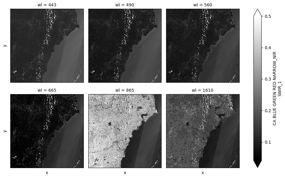
../_images/c4de5c40a239aff818df9210a39900bfeca9b5ce50d0da1391a2d0e772a38885.png

The reflectance data can also be easily plotted:

p = l1c.prod.bands.plot.imshow(col='wl', col_wrap=3,  vmax=0.5, robust=True, cmap=plt.cm.binary_r,subplot_kws=dict(xlabel='',xticks=[], yticks=[]))

../_images/180a0e5c0dd11ab53eddca1208fab45116a410bead86142e69c76b6d6f70baf3.png

For nicer plotting we use cartopy and argument ‘projection’ of matplotlib

import cartopy.crs as ccrs
str_epsg = str(l1c.epsg)
zone = str_epsg[-2:]
is_south = str_epsg[2] == 7
proj = ccrs.UTM(zone, is_south)

coarsening = 10
p = l1c.prod.sza[::coarsening, ::coarsening].plot.imshow(subplot_kws=dict(projection= proj), robust=True, cmap=plt.cm.Spectral_r)

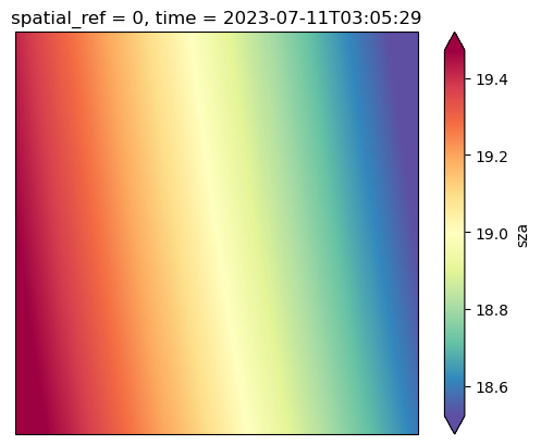
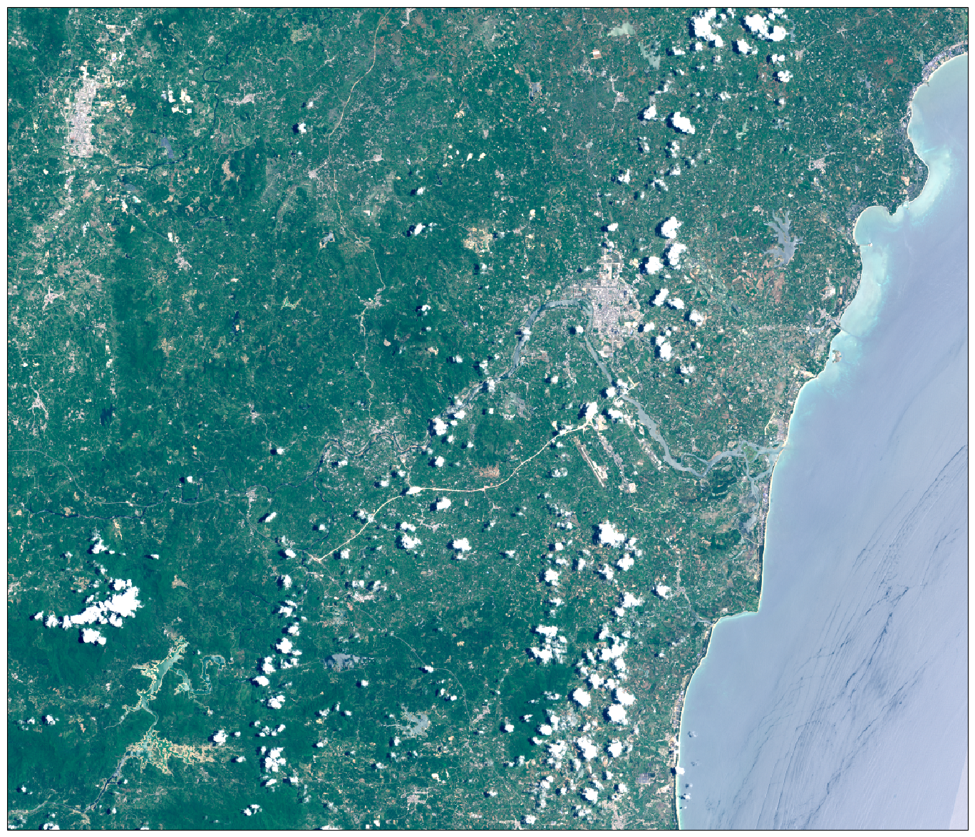
../_images/d8f4520c1c3a9c3887b42079c423cd9e9c716194b389398a0279cf404627f29d.png

And the RGB image:

# Get geographic projection and bounds
extent = l1c.extent

bounds = extent.bounds
extent_val = [bounds.minx[0], bounds.maxx[0]-40000, bounds.miny[0], bounds.maxy[0]-50000]
#extent_val = [bounds.minx[0], bounds.maxx[0], bounds.miny[0], bounds.maxy[0]]

fig = plt.figure(figsize=(20, 15))
ax = plt.subplot(1, 1, 1, projection=proj)
ax.set_extent(extent_val, proj)
coarsening=1
brightness_factor = 3.5
(l1c.prod.bands[:, ::coarsening, ::coarsening].sel(wl=[665,560,490])**0.5**brightness_factor
).plot.imshow(rgb='wl', robust=True,subplot_kws=dict(projection= proj))
ax.set_title('')

Text(0.5, 1.0, '')

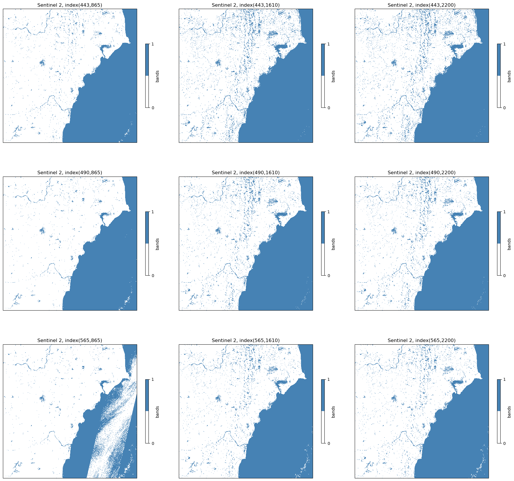
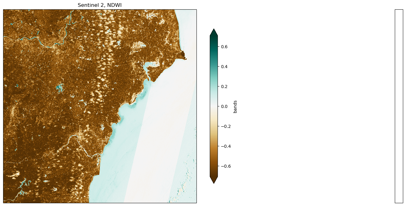
../_images/a41e85cdb50187b6e76b616d36e1a6701a62c190c3ded2ec3ca17e891347d7b9.png

Example of exploiation: compute NDWI for water pixel masking#

#coarsening to save memory and speed (if greater than 1)
coarsening=1


# binary cmap
bcmap = mpl.colors.ListedColormap([(0,0,0,0),'steelblue'])

def sindex(R1,R2):
    return (R1-R2)/(R1+R2) 
    
def water_mask(ndwi, threshold=0):
    water = xr.where(ndwi > threshold, 1, 0)
    return water.where(~np.isnan(ndwi))

def plot_water_mask(ndwi,ax,threshold=0):
    water = water_mask(ndwi, threshold)
   
    water.plot.imshow(ax=ax, transform=proj, cmap=bcmap,
                                  cbar_kwargs={'ticks': [0, 1], 'shrink': shrink})
    ax.set_title(str(threshold)+' < NDWI')

# Compute NDWI
green = l1c.prod.bands.sel(wl=565,method='nearest')
nir = l1c.prod.bands.sel(wl=865,method='nearest')
ndwi = (green - nir) / (green + nir)

fig = plt.figure(figsize=(20, 15))
fig.subplots_adjust(bottom=0.1, top=0.95, left=0.1, right=0.99,
                    hspace=0.05, wspace=0.05)
shrink = 0.8
    
ax = plt.subplot(2, 2, 1, projection=proj)
fig = ndwi[::coarsening, ::coarsening].plot.imshow( transform=proj, cmap=plt.cm.BrBG, robust=True,
                                   cbar_kwargs={'shrink': shrink})
# axes.coastlines(resolution='10m',linewidth=1)
ax.set_title('Sentinel 2, NDWI')

for i,threshold in enumerate([-0.2,0.,0.2]):
    ax = plt.subplot(2, 2, i+2, projection=proj)
    plot_water_mask(ndwi_,ax,threshold=threshold)

plt.show()

---------------------------------------------------------------------------
NameError                                 Traceback (most recent call last)
Cell In[22], line 19
     17 for i,threshold in enumerate([-0.2,0.,0.2]):
     18     ax = plt.subplot(2, 2, i+2, projection=proj)
---> 19     plot_water_mask(ndwi_,ax,threshold=threshold)
     21 plt.show()

NameError: name 'ndwi_' is not defined

../_images/542a1eab028072ab460284751bee379b9d492760acba5c53f5172328a6dc80a5.png

shrink = 0.4
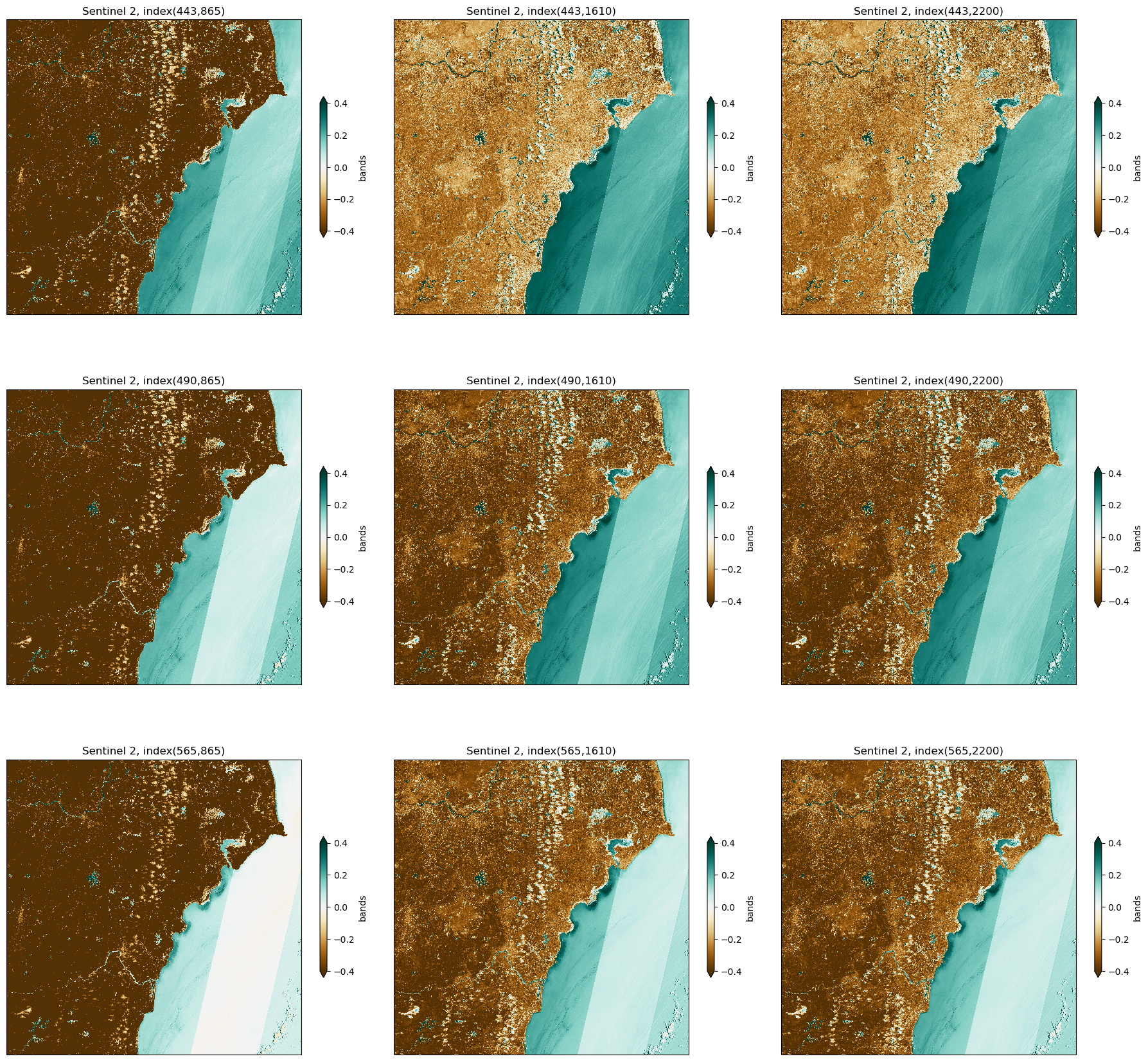
ii=1
ncols=3
nrows=3
fig,axs= plt.subplots(nrows,ncols,figsize=(20, 20),sharey=True,sharex=True,subplot_kw={'projection':proj})
fig.subplots_adjust(bottom=0.1, top=0.95, left=0.1, right=0.99,
                    hspace=0.05, wspace=0.05)
axs_=axs.ravel()
for bands in ([443,865],[443,1610],[443,2200],[490,865],[490,1610],[490,2200],[565,865],[565,1610],[565,2200]):
    #ax = plt.subplot(nrows,ncols, ii, projection=proj)
    
    ax=axs_[ii-1]

    fig = sindex(l1c.prod.bands.sel(wl=bands[0],method='nearest'),l1c.prod.bands.sel(wl=bands[1],method='nearest')).plot.imshow(ax=ax, transform=proj, cmap=plt.cm.BrBG, vmin=-0.4,robust=True,
                                       cbar_kwargs={'shrink': shrink})
    ax.set_title('Sentinel 2, index({:.0f},{:.0f})'.format(*bands))
    ii+=1

../_images/0ca2cd9491bb2dd297b9d9ac883bf1230b26ccab626af51a67ae2ad0aad24106.png

threshold=0
shrink = 0.4
ii=1
ncols=3
nrows=3
fig,axs= plt.subplots(nrows,ncols,figsize=(20, 20),sharey=True,sharex=True,subplot_kw={'projection':proj})
fig.subplots_adjust(bottom=0.1, top=0.95, left=0.1, right=0.99,
                    hspace=0.05, wspace=0.05)
axs_=axs.ravel()
for bands in ([443,865],[443,1610],[443,2200],[490,865],[490,1610],[490,2200],[565,865],[565,1610],[565,2200]):
    #ax = plt.subplot(nrows,ncols, ii, projection=proj)
    
    ax=axs_[ii-1]
    
    norm_index = sindex(l1c.prod.bands.sel(wl=bands[0],method='nearest'),l1c.prod.bands.sel(wl=bands[1],method='nearest'))
    plot_water_mask(norm_index,ax,threshold=threshold)
    ax.set_title('Sentinel 2, index({:.0f},{:.0f})'.format(*bands))
    ii+=1

Basics

Contents