Subsetting#
Notebook showing a fast and efficient way to load Sentinel-2 L1C data into xarray
import glob
import os
import numpy as np

import pandas as pd
import geopandas as gpd
import xarray as xr

import matplotlib.pyplot as plt
import matplotlib as mpl
import cartopy.crs as ccrs
from matplotlib.colors import ListedColormap

import GRSdriver
from GRSdriver import driver_S2_SAFE as S2

opj = os.path.join
print(f'-GRSdriver: {GRSdriver.__version__}')


-GRSdriver: 1.0.5
First, check the availbale bands:
S2.INFO
| bandId | 0 | 1 | 2 | 3 | 4 | 5 | 6 | 7 | 8 | 9 | 10 | 11 | 12 |
|---|---|---|---|---|---|---|---|---|---|---|---|---|---|
| ESA | B01 | B02 | B03 | B04 | B05 | B06 | B07 | B08 | B8A | B09 | B10 | B11 | B12 |
| EOREADER | CA | BLUE | GREEN | RED | VRE_1 | VRE_2 | VRE_3 | NIR | NARROW_NIR | WV | SWIR_CIRRUS | SWIR_1 | SWIR_2 |
| Wavelength (nm) | 443 | 490 | 560 | 665 | 705 | 740 | 783 | 842 | 865 | 945 | 1375 | 1610 | 2190 |
| Band width (nm) | 20 | 65 | 35 | 30 | 15 | 15 | 20 | 115 | 20 | 20 | 30 | 90 | 180 |
| Resolution (m) | 60 | 10 | 10 | 10 | 20 | 20 | 20 | 10 | 20 | 60 | 60 | 20 | 20 |
Choose the bands to be loaded (fill the bandIds array up) and the resolution between 10, 20 and 60 m:
# get all the 13 Sentinel-2 bands
bandIds = range(13) #[0,1,2,3,4,8,11,12]

resolution=20
datadir = '/data/satellite/Sentinel-2/L1C/'
odir = '/data/satellite/Sentinel-2/subset/L1C'
tile = '30PYT'
clon,clat = -0.66,11.6
width, height = 25000, 20000
complevel=5
test for one image#
file = '/data/satellite/Sentinel-2/L1C/30PYT/2021/11/17/S2B_MSIL1C_20211117T102219_N0500_R065_T30PYT_20221231T000708.SAFE'
year='2021'
Set the spatiotemporal utilitary to create a “bbox” from central longitude / latitude and extent
ust = GRSdriver.SpatioTemp()

box = ust.wktbox(clon, clat, width=width, height=height, ellps='WGS84')
bbox = gpd.GeoSeries.from_wkt([box]).set_crs(epsg=4326)
subset = bbox
subset
0    POLYGON ((-0.43062 11.78071, -0.88938 11.78071...
dtype: geometry
Naming of the output file and directory
file_nc = os.path.basename(file).replace('.SAFE', '.nc')
file_nc = opj(odir,tile,year,file_nc)
odir_ = os.path.dirname(file_nc)
Subset, compute angles and load into xarray dataset
l1c= S2.Sentinel2Driver(file,
                        band_idx=bandIds,
                        subset=subset,
                        resolution_angle=60,
                        resolution=resolution)
l1c.load_product()
/home/harmel/anaconda3/envs/grstbx/lib/python3.9/site-packages/xarray/core/indexes.py:659: RuntimeWarning: '<' not supported between instances of 'SpectralBandNames' and 'SpectralBandNames', sort order is undefined for incomparable objects.
  new_pd_index = pd_indexes[0].append(pd_indexes[1:])
str_epsg = str(l1c.prod.rio.crs)
zone = str_epsg[-2:]
is_south = str_epsg[2] == 7
proj = ccrs.UTM(zone, is_south)
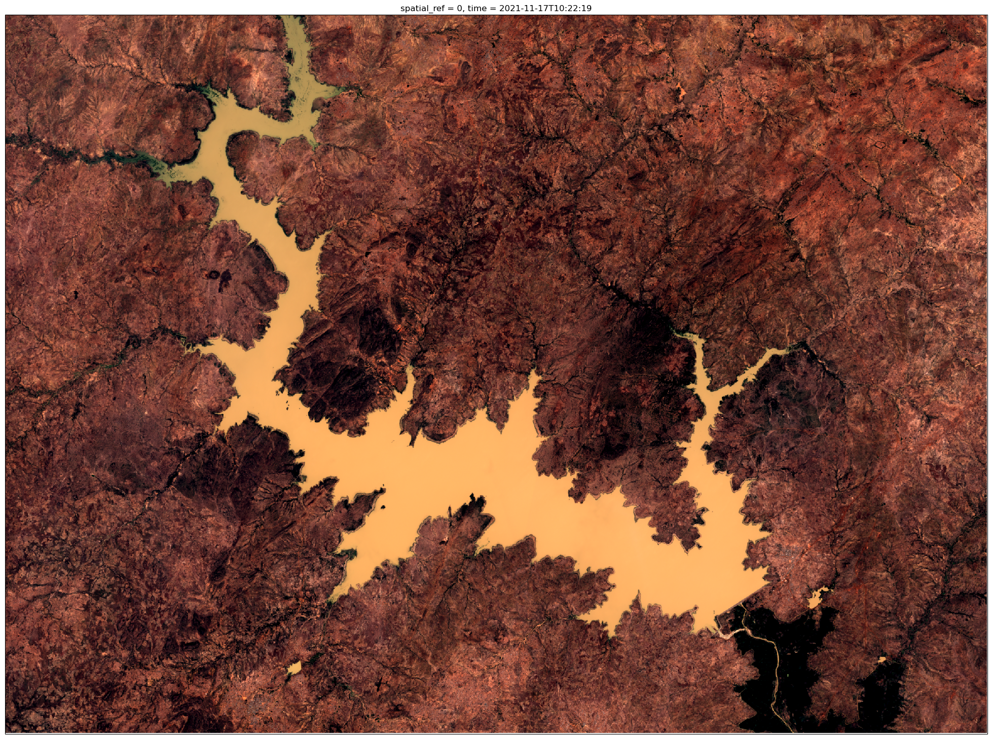
plt.figure(figsize=(25,25))
l1c.prod.bands.sel(wl=[665,560,490]).plot.imshow(rgb='wl', robust=True,subplot_kws=dict(projection=proj))
/home/harmel/anaconda3/envs/grstbx/lib/python3.9/site-packages/xarray/core/duck_array_ops.py:188: RuntimeWarning: overflow encountered in cast
  return data.astype(dtype, **kwargs)
<matplotlib.image.AxesImage at 0x7f40c5a4e490>
Encode and compress/save into netcdf file
encoding = {'bands': {'dtype': 'int16', 'scale_factor': 0.00005, 'add_offset': .3, '_FillValue': -32768,"zlib": True,
                                   "complevel": complevel, 'grid_mapping': 'spatial_ref'},
            'vza': {'dtype': 'int16', 'scale_factor': 0.01, '_FillValue': -9999,"zlib": True,
                                   "complevel": complevel, 'grid_mapping': 'spatial_ref'},
            'raa': {'dtype': 'int16', 'scale_factor': 0.1, '_FillValue': -9999,"zlib": True,
                                   "complevel": complevel, 'grid_mapping': 'spatial_ref'},
            'sza': {'dtype': 'int16', 'scale_factor': 0.01, '_FillValue': -9999,"zlib": True,
                                   "complevel": complevel, 'grid_mapping': 'spatial_ref'}
            }

if not os.path.exists(odir_):
    os.makedirs(odir_)

# l1c.prod.to_netcdf(file_nc, encoding=encoding)
Apply to a series of images#
year='2021'
datadir = '/data/satellite/Sentinel-2/L1C/'
odir = '/data/satellite/Sentinel-2/subset/L1C'
tile = '30PYT'
files = glob.glob(opj(datadir,tile,year,'*','*','*N05*SAFE'))
len(files)
47
ust = GRSdriver.SpatioTemp()

for file in files:

    box = ust.wktbox(clon, clat, width=width, height=height, ellps='WGS84')
    bbox = gpd.GeoSeries.from_wkt([box]).set_crs(epsg=4326)
    subset = bbox

    file_nc = os.path.basename(file).replace('.SAFE', '.nc')
    file_nc = opj(odir,tile,year,file_nc)
    odir_ = os.path.dirname(file_nc)

    if not os.path.exists(file_nc):
        print(file_nc)
    #if True:
        l1c= S2.Sentinel2Driver(file,
                                band_idx=bandIds,
                                subset=subset,
                                resolution_angle=60,
                                resolution=resolution)
        l1c.load_product()

        encoding = {'bands': {'dtype': 'int16', 'scale_factor': 0.00005, 'add_offset': .3, '_FillValue': -32768,"zlib": True,
                                           "complevel": complevel, 'grid_mapping': 'spatial_ref'},
                    'vza': {'dtype': 'int16', 'scale_factor': 0.01, '_FillValue': -9999,"zlib": True,
                                           "complevel": complevel, 'grid_mapping': 'spatial_ref'},
                    'raa': {'dtype': 'int16', 'scale_factor': 0.1, '_FillValue': -9999,"zlib": True,
                                           "complevel": complevel, 'grid_mapping': 'spatial_ref'},
                    'sza': {'dtype': 'int16', 'scale_factor': 0.01, '_FillValue': -9999,"zlib": True,
                                           "complevel": complevel, 'grid_mapping': 'spatial_ref'}
                    }


        if not os.path.exists(odir_):
            os.makedirs(odir_)
        l1c.prod.to_netcdf(file_nc, encoding=encoding)
        l1c.prod.close()
        del l1c
file_nc
'/data/satellite/Sentinel-2/subset/L1C/30PYT/2021/S2A_MSIL1C_20210923T102031_N0500_R065_T30PYT_20230121T095834.nc'
Create datacube#
files = glob.glob('/data/satellite/Sentinel-2/subset/L1C/30PYT/test/*nc')
datacube = xr.open_mfdataset(files,combine='nested',concat_dim='time')
datacube
<xarray.Dataset>
Dimensions:      (x: 2526, y: 1653, wl: 13, time: 22, wl_hr: 1950)
Coordinates:
  * x            (x) float64 7.298e+05 7.299e+05 ... 7.803e+05 7.804e+05
  * y            (y) float64 1.3e+06 1.3e+06 1.3e+06 ... 1.267e+06 1.267e+06
    spatial_ref  int64 0
  * wl           (wl) int64 443 490 560 665 705 740 ... 865 945 1375 1610 2190
  * wl_hr        (wl_hr) int64 400 401 402 403 404 ... 2345 2346 2347 2348 2349
  * time         (time) datetime64[ns] 2021-06-15T10:20:21 ... 2021-06-05T10:...
Data variables:
    bands        (time, wl, y, x) float32 dask.array<chunksize=(1, 13, 1653, 2526), meta=np.ndarray>
    SRF          (time, wl, wl_hr) float64 dask.array<chunksize=(1, 13, 1950), meta=np.ndarray>
    wl_true      (time, wl) float64 dask.array<chunksize=(1, 13), meta=np.ndarray>
    vza          (time, wl, y, x) float32 dask.array<chunksize=(1, 13, 1653, 2526), meta=np.ndarray>
    raa          (time, wl, y, x) float32 dask.array<chunksize=(1, 13, 1653, 2526), meta=np.ndarray>
    sza          (time, y, x) float32 dask.array<chunksize=(1, 1653, 2526), meta=np.ndarray>
Attributes: (12/50)
    long_name:                           CA BLUE GREEN RED VRE_1 VRE_2 VRE_3 ...
    constellation:                       Sentinel-2
    constellation_id:                    S2
    product_path:                        /data/satellite/Sentinel-2/L1C/30PYT...
    product_name:                        S2A_MSIL1C_20210615T102021_N0500_R06...
    product_filename:                    S2A_MSIL1C_20210615T102021_N0500_R06...
    ...                                  ...
    satellite:                           S2A
    tile:                                30PYT
    solar_irradiance:                    [1884.69 1959.66 1823.24 1512.06 142...
    solar_irradiance_unit:               W/m²/µm
    mean_solar_azimuth:                  56.429553875236294
mean_solar_zenith_angle: 23.604009829867675Plotting section#
The MSI-Sentinel-2 instrument is composed of 12 detectors staggered in two different rows making a “switch” in viewng geometries along the image especially for the azimuth values. Here, we plot the solar and viewing zenith angles as well as the relative azimuth between Sun and sensor directions. The sun viewing angle (SZA) is common to all the spectral bands.
Set ‘reproject=True’ to repoject raster into WGS 84 / Pseudo-Mercator for web mapping and visualization (e.g., OpenStreetMap). The EPSG code is 3857.
datacube.bands.load()
h=GRSdriver.ViewSpectral(datacube.bands.sortby('time'),reproject=True)#.assign_coords(time=l1c.datetime).expand_dims('time')
# h.colormaps = ['CET_D13', 'bky', 'CET_D1A','CET_CBL2','CET_L10','CET_C6s', 'kbc', 'blues_r', 'kb', 'rainbow', 'fire', 'kgy', 'bjy','gray' ]
h.visu()
Uncomment next cell for pratical use
#geom_ = h.get_geom(h.aoi_stream,crs=datacube.rio.crs)
#geom_.to_file("roi_test.json", driver="GeoJSON")
geom_ = gpd.read_file("roi_test.json", driver="GeoJSON")
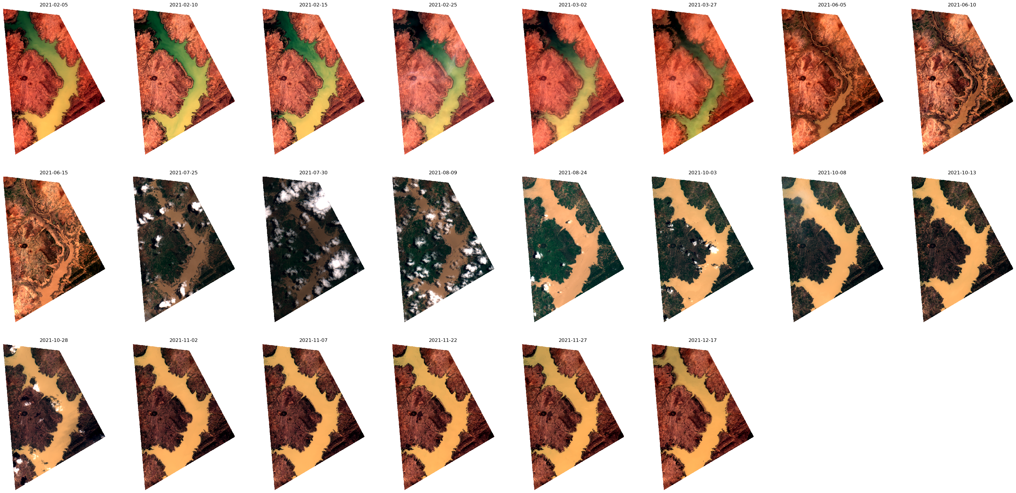
Rtoa_clipped = datacube.bands.rio.clip(geom_.geometry.values)
RGB = Rtoa_clipped.isel(wl=[3,2,1])#.isel(time=[0,1,2,3])

str_epsg = str(RGB.rio.crs)
zone = str_epsg[-2:]
is_south = str_epsg[2] == 7
proj = ccrs.UTM(zone, is_south)

ncols=8

dates =  RGB.time

Ndates = len(dates.values)
ncols=np.min([ncols,Ndates])
nrows=int(np.ceil(Ndates/ncols))

fig,axs = plt.subplots(nrows,ncols,figsize=(ncols*4.9,5*nrows+5),subplot_kw={'projection': proj})
fig.subplots_adjust(bottom=0.08, top=0.9, left=0.086, right=0.98,
                    hspace=0.15, wspace=0.07,)
if (ncols == 1) & (nrows == 1):
    axs = np.array([axs])
axs=axs.ravel()
[axi.set_axis_off() for axi in axs]
for ii,(date, xraster_) in enumerate(RGB.groupby('time')):
    date = pd.to_datetime(str(date))
    date_ = date.strftime('%Y-%m-%d')

    xraster_.squeeze().plot.imshow(rgb='wl',ax=axs[ii],robust=True)
    axs[ii].set_title(date_)
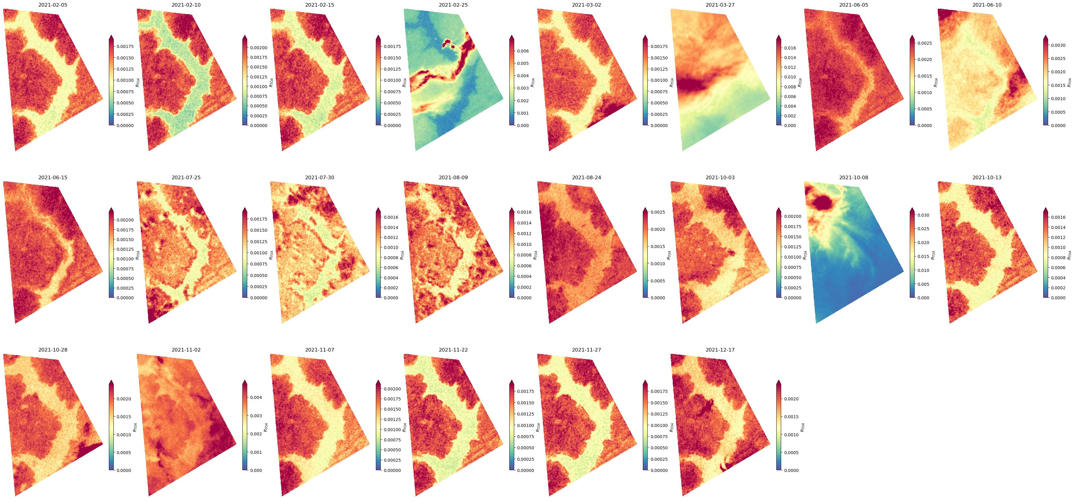
band = Rtoa_clipped.isel(wl=10)#.isel(time=[0,1,2,3])

str_epsg = str(band.rio.crs)
zone = str_epsg[-2:]
is_south = str_epsg[2] == 7
proj = ccrs.UTM(zone, is_south)

ncols=8

dates =  band.time

Ndates = len(dates.values)
ncols=np.min([ncols,Ndates])
nrows=int(np.ceil(Ndates/ncols))

fig,axs = plt.subplots(nrows,ncols,figsize=(ncols*4.9,5*nrows+5),subplot_kw={'projection': proj})
fig.subplots_adjust(bottom=0.08, top=0.9, left=0.086, right=0.98,
                    hspace=0.15, wspace=0.07,)
if (ncols == 1) & (nrows == 1):
    axs = np.array([axs])
axs=axs.ravel()
[axi.set_axis_off() for axi in axs]
for ii,(date, xraster_) in enumerate(band.groupby('time')):
    date = pd.to_datetime(str(date))
    date_ = date.strftime('%Y-%m-%d')

    xraster_.squeeze().plot.imshow(cmap=plt.cm.Spectral_r,ax=axs[ii],robust=True,vmin=0,cbar_kwargs={ 'shrink':0.6,'label':'$R_{TOA}$'})
    axs[ii].set_title(date_)